Processing math: 100%

Predicting Subglacial Lakes in Antarctica

Jake Bova | Programming for Geographic Information Systems | Fall 2024

We know: Subglacial lakes are present in Antarctica.

We want to know: Where are they?

Hypothesis: Subglacial lakes are more likely to be present in specific regions of Antarctica.

Using various geospatial raster datasets, I will predict the possible presence of subglacial lakes in Antarctica.

Primary Sources

• Wright A, Siegert M. A fourth inventory of Antarctic subglacial lakes. Antarctic Science. 2012
  • https://www.cambridge.org/core/journals/antarctic-science/article/fourth-inventory-of-antarctic-subglacial-lakes/81B35C31B0DFCE1B3A0705B779D3AF58
• Davies B. Antarctic Subglacial Lakes. AntarcticGlaciers.org. June 22, 2020
  • https://www.antarcticglaciers.org/glacier-processes/glacial-lakes/subglacial-lakes/
• Livingstone SJ. et al. Potential Subglacial Lake locations and meltwater drainage pathways beneath the Antarctic and Greenland Ice Sheets. The Cryosphere. 2013;7(6):1721-1740. doi:10.5194/tc-7-1721-2013
  • https://tc.copernicus.org/articles/7/1721/2013/tc-7-1721-2013.pdf
• Goeller S. et al. Assessing the Subglacial Lake coverage of Antarctica. Annals of Glaciology. 2016
  • https://www.cambridge.org/core/journals/annals-of-glaciology/article/assessing-the-subglacial-lake-coverage-of-antarctica/735373D91B8BAB10196D96820A4E93B0

Package Imports

import pandas as pd
import numpy as np
import matplotlib.pyplot as plt
import geopandas as gpd

import raster_tools as rt

from sklearn.ensemble import RandomForestClassifier, IsolationForest
from sklearn.preprocessing import StandardScaler
from sklearn.model_selection import train_test_split
from sklearn.metrics import classification_report, confusion_matrix, roc_curve, auc
import seaborn as sns
from pathlib import Path
import time
import datetime

# supress all warnings
import warnings
warnings.filterwarnings("ignore")

Data

WEB RASTERS (IMPORTANT): https://umontana.maps.arcgis.com/apps/instant/imageryviewer/index.html?appid=88c564444ef744f1a16095c1dc358eb6

QUANTARCTICA: https://www.npolar.no/quantarctica/

Input Data

Name	Type	Info	Grid Size	Source
known_lakes	Vector	GDF of known lakes	1km	Wright, A., and Siegert, M. (2012)
lakes_raster	Vector/Raster	Rasterized known lake points	1km	Wright, A., and Siegert, M. (2012)
dem	Raster	Digitel elevation model	1km	BEDMAP2 (Fretwell et al., BAS/The Cryosphere, 2013)
slope	Raster	DEM Slope	1km	BEDMAP2 (derived)
ice_thickness	Raster	Ice sheet thickness	1km	BEDMAP2 (Fretwell et al., BAS/The Cryosphere, 2013)
bed_elevation	Raster	DEM of Antarctic bed	1km	BEDMAP2 (Fretwell et al., BAS/The Cryosphere, 2013)
bed_slope	Raster	DEM Bed Slope	1km	BEDMAP2 (derived, raster_tools)
bed_flow_dir	Raster	Bed flow direction	1km	BEDMAP2 (derived, QGIS)
bed_flow_acc	Raster	Bed flow accumulation	1km	BEDMAP2 (derived, QGIS)
hp_flow_acc	Raster	Hydraulic Flow Acc. Gradient (log)	1km	BEDMAP2 (derived from bed_elevation and ice_thickness, Shreve equation implemented using raster_tools)
ice_bound_prox	Vector/Raster	Global Promity to ice boundary	1km	MEaSUREs Antarctic boundaries (rasterized and calculated with raster_tools)
radarsat	Raster	Radar backscatter imagery	100m	RAMP RADARSAT mosaic (Jezek et al., NSIDC, 1999/2013) (reprojected and warped with raster_tools to DEM 1km grid)
ice_velocity	Raster	X and Y velocity in m/yr	450m	MEaSUREs Antarctic velocity map v2 (Rignot et al., NSIDC, 2017) (reprojected and warped with raster_tools to DEM 1km grid)
subglacial_water_flux	Raster	Modelled subglacial water flux beneath the grounded ice sheet	1km	Le Brocq et al., Nature Geoscience, 2013, derived from BEDMAP2
prox_to_known_lake	Raster	Global Proximity to known lake points	1km	Wright, A., and Siegert, M. (2012), calculated with raster_tools
possible_lake_areas	Raster	Filtered raster from slope and ice_bound_prox	1km	Jake Bova (2024)

Shreve's Equation: $$\text{Hydraulic Potential} = \rho_w g h + \rho_i g H$$ Where:

• $\rho_w$ = density of water
• $g$ = acceleration due to gravity
• $h$ = bed elevation
• $\rho_i$ = density of ice
• $H$ = ice thickness

Original possible lake areas from Jake Bova (2024) are filtered by slope < ~0.1 and proximity to ice boundary < 200km to create possible_lake_areas.

This is a simple method but it is was good starting point for further analysis.

Data Processing

def load_lake_data(lake_path):
    """Load and preprocess lake data"""
    lakes = gpd.read_file(lake_path)
    # Clean LENGTH_M column
    lakes['LENGTH_M'] = (lakes['LENGTH_M']
                        .str.replace('28100 + 4000', '28100')
                        .str.replace('<', '')
                        .str.replace(' ', ''))
    lakes['LENGTH_M'] = pd.to_numeric(lakes['LENGTH_M'], errors='coerce')
    lakes['SAT_DETECT'] = np.where(lakes['CLASS'] == 'G', 1, 0)
    return lakes

def load_raster_data(config):
    """Load all raster data based on configuration dictionary"""
    rasters = {}
    for name, path in config['raster_paths'].items():
        try:
            rasters[name] = rt.Raster(path)
        except Exception as e:
            print(f"Error loading {name}: {e}")
    
    # Handle derived rasters
    if 'bed_slope' not in rasters and 'bed_elevation' in rasters:
        rasters['bed_slope'] = rt.surface.slope(rasters['bed_elevation'])
    if 'slope' not in rasters and 'dem' in rasters:
        rasters['slope'] = rt.surface.slope(rasters['dem'])
    
    # Special processing for subglacial water flux
    if 'subglacial_water_flux' in rasters:
        rasters['subglacial_water_flux'] = process_water_flux(rasters['subglacial_water_flux'])
    
    return rasters

def process_water_flux(water_flux):
    """Process subglacial water flux data"""
    water_flux = np.log10(water_flux + 1)
    return water_flux.where(water_flux != -np.inf, other=np.nan)

def find_threshold_areas(slope, hp_flow_acc, ice_bound_prox):
    """Identify possible lake areas based on thresholds"""
    condition1 = slope < 0.15  # 0.15 degrees angle
    condition2 = (hp_flow_acc > 6) & (hp_flow_acc < 10)
    condition3 = ice_bound_prox < 200000
    
    combined_mask = condition1 & condition2 & condition3
    return combined_mask.astype('uint8')

def reproject_rasters(rasters, template_raster, config):
    """Reproject rasters to match template"""
    for name in config['needs_reprojection']:
        if name in rasters:
            rasters[name] = rt.warp.reproject(
                rasters[name], 
                template_raster.crs,
                resample_method='bilinear',
                resolution=1000
            )
    return rasters

def clip_rasters(rasters, clip_geometry):
    """Clip all rasters to geometry"""
    return {name: rt.clipping.clip(clip_geometry, raster) 
            for name, raster in rasters.items()}

def vectorize_rasters(rasters):
    """Convert rasters to vectors"""
    vectors = {}
    for name, raster in rasters.items():
        vectors[name] = raster.to_vector().compute()
        if 'band' in vectors[name].columns:
            vectors[name].drop(columns=['band', 'row', 'col'], inplace=True)
        
        # Add coordinates for specific layers
        if name in ['radarsat', 'ice_velocity']:
            vectors[name]['x_m'] = vectors[name].geometry.x
            vectors[name]['y_m'] = vectors[name].geometry.y
            
            # Apply offsets
            if name == 'radarsat':
                vectors[name]['x_m'] -= 50
                vectors[name]['y_m'] += 50
            elif name == 'ice_velocity':
                vectors[name]['x_m'] -= 275
                vectors[name]['y_m'] -= 725
    
    return vectors

def merge_vectors(vectors, config):
    """Merge all vector data"""
    merged = None
    
    for step in config['merge_steps']:
        left = vectors[step['left']]
        right = vectors[step['right']]
        
        if step.get('spatial', True):
            merged = gpd.sjoin(
                left if merged is None else merged,
                right,
                how=step.get('how', 'inner'),
                op='intersects',
                rsuffix=f"_{step['right']}"
            )
        else:
            merged = merged.merge(
                right,
                on=step.get('on', ['x_m', 'y_m']),
                how=step.get('how', 'inner')
            )
        
        if 'drop_columns' in step:
            merged.drop(columns=step['drop_columns'], inplace=True)
        if 'rename_columns' in step:
            merged.rename(columns=step['rename_columns'], inplace=True)
            
    # Post-processing
    if 'known_lake' in merged.columns:
        merged['possible_lake_area'] = np.where(
            merged.known_lake == 1, 
            1, 
            merged.possible_lake_area
        )
    
    return merged

def get_data():
    # Configuration
    config = {
        'raster_paths': {
            'dem': 'data/Quantarctica3/Quantarctica3/TerrainModels/BEDMAP2/bedmap2_surface.tif',
            'bed_elevation': 'data/Quantarctica3/Quantarctica3/TerrainModels/BEDMAP2/bedmap2_bed.tif',
            'ice_thickness': 'data/Quantarctica3/Quantarctica3/TerrainModels/BEDMAP2/bedmap2_thickness.tif',
            'bed_flow_dir': 'data/bed_flow_dir.tif',
            'bed_flow_acc': 'data/bed_flow_acc.tif',
            'hp_flow_acc': 'data/ant_flow_acc_log10.tif',
            'radarsat': 'data/Quantarctica3/Quantarctica3/SatelliteImagery/RADARSAT/RADARSAT_Mosaic.jp2',
            'ice_velocity': 'input_data/icevel_filled.tif',
            'subglacial_water_flux': 'data/Quantarctica3/Quantarctica3/Glaciology/Subglacial Water Flux/SubglacialWaterFlux_Modelled_1km.tif'
        },
        'needs_reprojection': ['radarsat', 'ice_velocity'],
        'merge_steps': [
            {
                'left': 'slope',
                'right': 'dem',
                'rename_columns': {'value_slope': 'slope', 'value_dem': 'dem'},
                'drop_columns': ['band_slope', 'row_slope', 'col_slope', 'index_dem', 'band_dem', 'row_dem', 'col_dem']
            },
            {
                'left': 'merged',
                'right': 'ice_thickness',
                'rename_columns': {'value': 'ice_thickness'}
            },
            {
                'left': 'merged',
                'right': 'bed_elevation',
                'rename_columns': {'value': 'bed_elevation'},
                'drop_columns': ['index_ice_thickness', 'band_left', 'row_left', 'col_left', 
                               'index_bed_elevation', 'band_bed_elevation', 'row_bed_elevation', 'col_bed_elevation']
            },
            {
                'left': 'merged',
                'right': 'bed_slope',
                'rename_columns': {'value': 'bed_slope'},
                'drop_columns': ['index_bed_slope', 'band', 'row', 'col']
            },
            {
                'left': 'merged',
                'right': 'bed_flow_dir',
                'rename_columns': {'value': 'bed_flow_dir'},
                'drop_columns': ['index_bed_flow_dir', 'band', 'row', 'col']
            },
            {
                'left': 'merged',
                'right': 'bed_flow_acc',
                'rename_columns': {'value': 'bed_flow_acc'},
                'drop_columns': ['index_bed_flow_acc', 'band', 'row', 'col']
            },
            {
                'left': 'merged',
                'right': 'hp_flow_acc',
                'rename_columns': {'value': 'hp_flow_acc_log'},
                'drop_columns': ['index_hp_flow_acc', 'band', 'row', 'col']
            },
            {
                'left': 'merged',
                'right': 'prox_to_known_lake',
                'rename_columns': {'value': 'prox_to_known_lake_m'},
                'drop_columns': ['index_prox_to_known_lake', 'band', 'row', 'col']
            },
            {
                'left': 'merged',
                'right': 'ice_bound_prox',
                'rename_columns': {'value': 'ice_bound_prox_m'},
                'drop_columns': ['index_ice_bound_prox', 'band', 'row', 'col']
            },
            {
                'left': 'merged',
                'right': 'lakes',
                'how': 'left',
                'rename_columns': {'value': 'known_lake'},
                'drop_columns': ['index_lakes', 'band', 'row', 'col']
            },
            {
                'left': 'merged',
                'right': 'possible_lake_areas',
                'rename_columns': {'value': 'possible_lake_area'},
                'drop_columns': ['index_possible_lake_areas', 'band', 'row', 'col']
            },
            {
                'left': 'merged',
                'right': 'subglacial_water_flux',
                'rename_columns': {'value': 'subglacial_water_flux'},
                'drop_columns': ['index_subglacial_water_flux', 'band', 'row', 'col']
            },
            {
                'left': 'merged',
                'right': 'radarsat',
                'spatial': False,
                'rename_columns': {'value': 'radarsat', 'geometry_x': 'geometry'},
                'drop_columns': ['geometry_y']
            },
            {
                'left': 'merged',
                'right': 'ice_velocity',
                'spatial': False,
                'rename_columns': {'value': 'ice_vel', 'geometry_x': 'geometry'},
                'drop_columns': ['geometry_y']
            }
        ]
    }
    
    # Load and process data
    lakes = load_lake_data('data/Quantarctica3/Quantarctica3/Glaciology/Subglacial Lakes/SubglacialLakes_WrightSiegert.shp')
    rasters = load_raster_data(config)
    
    # Load world boundary for clipping
    world = gpd.read_file('data/Quantarctica3/Quantarctica3/Miscellaneous/SimpleBasemap/ADD_DerivedLowresBasemap.shp')
    world = world.to_crs(epsg=3031)
    world_land = world[world['Category'] == 'Land']
    
    # Process rasters
    rasters = reproject_rasters(rasters, rasters['dem'], config)
    
    # Calculate possible lake areas
    rasters['possible_lake_areas'] = find_threshold_areas(
        rasters['slope'],
        rasters['hp_flow_acc'],
        rasters['ice_bound_prox']
    )
    
    # Clip and vectorize
    clipped_rasters = clip_rasters(rasters, world_land)
    vectors = vectorize_rasters(clipped_rasters)
    
    # Merge data
    merged = merge_vectors(vectors, config)
    
    # Final processing
    merged = gpd.GeoDataFrame(merged, geometry='geometry')
    merged.set_crs(epsg=3031, inplace=True)
    
    # Clean up
    merged = merged.dropna(subset=['slope'])
    merged['subglacial_water_flux'] = merged['subglacial_water_flux'].fillna(
        merged['subglacial_water_flux'].mean()
    )
    merged = merged.dropna(subset=['subglacial_water_flux'])
    
    return merged

# merged = get_data() # Load data
merged = pd.read_csv('input_data/merged_data.csv')
merged = gpd.GeoDataFrame(merged, geometry=gpd.points_from_xy(merged.x_m, merged.y_m))
merged.set_crs(epsg=3031, inplace=True)
merged.drop(columns=['Unnamed: 0'], inplace=True)
df = merged.drop(columns=['geometry', 'prox_to_known_lake_m', 'possible_lake_area', 'x_m', 'y_m']) # Drop geometry and other columns for training (x_m and y_m were used for merging)
df_known_lakes = df[df['known_lake'] == 1]

After preparing the data we get a geodataframe of every raster point covered by BEDMAP2.

I decided to not use proximity to known lakes as a feature because it is basically the same as the known_lakes raster (with 0 distance being a known lake).

df

	slope	dem	ice_thickness	bed_elevation	bed_slope	bed_flow_dir	bed_flow_acc	hp_flow_acc_log	ice_bound_prox_m	known_lake	subglacial_water_flux	radarsat	ice_vel
0	0.707877	51	168	-117	0.780114	8	2.0	5.560527	1000.0000	0	0.0	218	9.844176
1	0.810800	56	164	-108	0.683401	8	3.0	5.981568	1000.0000	0	0.0	220	3.164224
2	0.907321	60	162	-102	0.567633	8	3.0	6.260069	1414.2136	0	0.0	223	2.593423
3	0.999757	62	160	-98	0.489942	8	0.0	6.478846	1414.2136	0	0.0	224	3.497082
4	1.088866	63	160	-97	0.452274	4	0.0	6.663968	1000.0000	0	0.0	224	3.351763
...	...	...	...	...	...	...	...	...	...	...	...	...	...
11859923	3.375342	158	344	-186	3.351585	4	3.0	6.926358	1000.0000	0	0.0	217	8.147156
11859924	3.489445	178	339	-161	3.467022	4	2.0	6.784882	1000.0000	0	0.0	206	5.284122
11859925	3.480071	192	334	-142	3.459608	4	1.0	6.977334	1414.2136	0	0.0	208	3.320855
11859926	3.348109	198	327	-129	3.278850	4	0.0	6.818604	1000.0000	0	0.0	214	2.504690
11859927	3.147901	192	321	-129	3.007938	4	0.0	6.210092	1000.0000	0	0.0	222	2.143291

11859928 rows × 13 columns

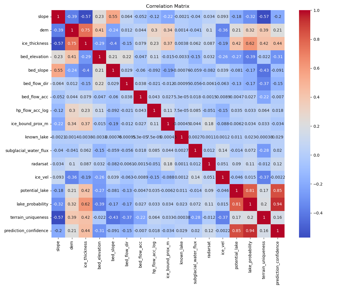
Many features correlate with each other, as can be seen from the correlation matrix below. This is expected as geospacial data is often highly correlated, and many of the features are derived from the same data.

df_no_lakes = df.drop(columns=['known_lake'])
corr = df_no_lakes.corr()
plt.figure(figsize=(12, 10))
sns.heatmap(corr, annot=True, cmap='coolwarm', center=0)
plt.show()

We can also inspect the distribution of data in known lake areas vs the rest of the data.

fig, axes = plt.subplots(4, 3, figsize=(15, 15))
cols = df.columns
cols = cols.drop('known_lake')
for i, col in enumerate(cols):
   ax = axes[i // 3, i % 3]
   
   # Calculate statistics
   stats_all = {
       'mean': df[col].mean(),
       'median': df[col].median(),
       'min': df[col].min(),
       'max': df[col].max()
   }
   
   stats_known = {
       'mean': df_known_lakes[col].mean(),
       'median': df_known_lakes[col].median(),
       'min': df_known_lakes[col].min(),
       'max': df_known_lakes[col].max()
   }
   
   # Plot histograms
   ax.hist(df[col], bins=50, alpha=0.5, label='All', log=True, color='orange')
   ax.hist(df_known_lakes[col], bins=50, alpha=0.5, label='Known Lakes', log=True, color='blue')
   
   # Add title and legend
   ax.set_title(col)
   ax.legend(loc='upper right')
   
   # Create and add text blocks separately with different colors
   all_text = (
       f"All Data (orange):\n"
       f"  Mean: {stats_all['mean']:.2f}\n"
       f"  Median: {stats_all['median']:.2f}\n"
       f"  Range: [{stats_all['min']:.2f}, {stats_all['max']:.2f}]"
   )
   
   known_text = (
       f"\n\nKnown Lakes (blue):\n"
       f"  Mean: {stats_known['mean']:.2f}\n"
       f"  Median: {stats_known['median']:.2f}\n"
       f"  Range: [{stats_known['min']:.2f}, {stats_known['max']:.2f}]"
   )
   
   # Add text blocks with separate colors
   ax.text(0.05, 0.95, all_text,
           transform=ax.transAxes,
           verticalalignment='top',
           fontsize=8,
           family='monospace',
           color='orange',
           bbox=dict(facecolor='white', alpha=0.8))
           
   ax.text(0.05, 0.65, known_text,
           transform=ax.transAxes,
           verticalalignment='top',
           fontsize=8,
           family='monospace',
           color='blue',
           bbox=dict(facecolor='white', alpha=0.8))

plt.tight_layout()
plt.show()

As you can see, the data for known lake locations follows a similar distribution to the rest of the data, but is skewed towards extreme values across almost all features.

Model Creation

I decided to use a Random Forest model, as it is a good starting point for geospatial data and I have had success with it in the past.

Simple initial model

# simple random forest model to predict known_lake
# we will have to oversample the known_lake = 1 class
from sklearn.ensemble import RandomForestClassifier
from sklearn.model_selection import train_test_split
from sklearn.metrics import classification_report, confusion_matrix

# first, drop n percent of the data that has known_lake = 0
df_sample = df.sample(frac=0.2)

# add back the known_lakes 10 times
for i in range(10):
    df_sample = pd.concat([df_sample, df_known_lakes])

X = df_sample.drop(columns=['known_lake'])
y = df_sample['known_lake']

X_train, X_test, y_train, y_test = train_test_split(X, y, test_size=0.3)

# oversample the known_lake = 1 class
from imblearn.over_sampling import SMOTE

# sm = SMOTE(random_state=42)
# X_train, y_train = sm.fit_resample(X_train, y_train)

clf = RandomForestClassifier(n_estimators=100)
clf.fit(X_train, y_train)
y_pred = clf.predict(X_test)

print(confusion_matrix(y_test, y_pred))
print(classification_report(y_test, y_pred))

# get column names and then list the feature importances
feature_importances = clf.feature_importances_
feature_names = X.columns
feature_importances_df = pd.DataFrame({'feature': feature_names, 'importance': feature_importances})
feature_importances_df = feature_importances_df.sort_values('importance', ascending=False)
feature_importances_df

Enhanced model

def prepare_data(df, sample_frac=0.05, known_lakes_multiplier=10):
    """
    Prepare training data with balanced representation of known lakes and non-lake areas
    
    Args:
        df: Input dataframe containing lake and terrain features
        sample_frac: Fraction of non-lake data to sample (reduces class imbalance)
        known_lakes_multiplier: Number of times to duplicate known lake data (further balances classes)
    """
    # Take a random sample of the full dataset to reduce computational load and class imbalance
    df_sample = df.sample(frac=sample_frac, random_state=42)
    
    # Extract all known lake locations
    df_known_lakes = df[df['known_lake'] == 1]
    
    # Since we are sampling such a small fraction of the data, we need to balance the classes
    # I was using SMOTE before, but just duplicating the known lakes is simpler and works well
    # It does cause some overfitting, but that is kind of the point here (we want to find lakes)
    # Duplicate known lakes multiple times to balance the dataset
    # This helps prevent the model from being biased towards the majority class (non-lakes)
    for i in range(known_lakes_multiplier):
        df_sample = pd.concat([df_sample, df_known_lakes])

    # Remove any rows with missing values to ensure clean training data
    df_sample.dropna(inplace=True)
    
    return df_sample

def train_anomaly_detector(X_train, contamination=0.01):
    """
    Train an isolation forest to detect unusual terrain features
    The idea here is to identify areas that are unique compared to the rest of the dataset.
    Imagine this as a way to find "hidden lakes" that are not easily classified by the main model.
    The basic idea is that if a location is very different from the rest of the terrain, it might be a lake (naive assumption).
    We basically look at every feature of a data point and see how different it is from the rest of the dataset.
    
    Args:
        X_train: Training data with terrain features
        contamination: Expected proportion of anomalies in the dataset
    """
    # Initialize isolation forest with specified contamination rate
    # Contamination represents expected proportion of outliers in the dataset
    iso_forest = IsolationForest(contamination=contamination, random_state=42)
    
    # Fit the model to learn what "normal" terrain looks like
    iso_forest.fit(X_train)
    return iso_forest

def create_lake_prediction_model(df, features_to_exclude=None, data_frac=0.05):
    """
    Create and train both the main classifier and anomaly detector
    
    Args:
        df: Input dataframe with all features
        features_to_exclude: List of columns to exclude from training
        data_frac: Fraction of data to use for training
    """
    # Get balanced dataset for training
    df_sample = prepare_data(df, sample_frac=data_frac)
    
    # Separate features and target variable
    X = df_sample.drop(columns=features_to_exclude if features_to_exclude else [])
    y = df_sample['known_lake']
    
    # Standardize features to ensure all are on same scale
    scaler = StandardScaler()
    X_scaled = scaler.fit_transform(X)
    X_scaled = pd.DataFrame(X_scaled, columns=X.columns)
    
    # Split data into training and testing sets
    X_train, X_test, y_train, y_test = train_test_split(X_scaled, y, test_size=0.3, random_state=42)
    
    # Initialize and train Random Forest classifier with parameters tuned for imbalanced data
    clf = RandomForestClassifier(n_estimators=200,  # Number of trees
                               max_depth=10,         # Maximum depth of trees (prevents overfitting)
                               min_samples_split=5,  # Minimum samples needed to split a node
                               class_weight='balanced',  # Adjusts weights inversely proportional to class frequencies
                               random_state=42)
    clf.fit(X_train, y_train)
    
    # Train anomaly detector on same training data
    iso_forest = train_anomaly_detector(X_train)
    
    return clf, iso_forest, scaler, X_test, y_test

def predict_potential_lakes(df, clf, iso_forest, scaler, features_to_exclude=None, 
                          similarity_threshold=0.3, anomaly_threshold=-0.5):
    """
    Combine classifier and anomaly detection predictions to identify potential lakes
    
    Args:
        similarity_threshold: Minimum probability threshold for lake classification
        anomaly_threshold: Minimum score for terrain uniqueness
    """
    # Clean and prepare prediction data
    df.dropna(inplace=True)
    X_pred = df.drop(columns=features_to_exclude if features_to_exclude else [])
    X_pred_scaled = scaler.transform(X_pred)
    
    # Get probability predictions from random forest (how likely is this a lake?)
    lake_probabilities = clf.predict_proba(X_pred_scaled)[:, 1]
    
    # Get anomaly scores (how unique is this terrain?)
    anomaly_scores = iso_forest.score_samples(X_pred_scaled)
    
    # Combine predictions: location must have both high lake probability and unique terrain
    potential_lakes = (lake_probabilities > similarity_threshold) & (anomaly_scores < anomaly_threshold) # swapped from > to <, because anomaly score is negative, meaning lower is more unique
    
    return potential_lakes, lake_probabilities, anomaly_scores

def analyze_predictions(df, potential_lakes, lake_probabilities, anomaly_scores, iteration=None):
    """
    Combine predictions and calculate confidence scores
    
    Args:
        iteration: Used for iterative confidence weighting (optional)
    """
    # Copy input data to avoid modifications
    df_results = df.copy()
    
    # Add prediction results as new columns
    df_results['potential_lake'] = potential_lakes
    df_results['lake_probability'] = lake_probabilities
    df_results['terrain_uniqueness'] = anomaly_scores
    
    # Calculate confidence score as weighted combination of lake probability and terrain uniqueness
    df_results['prediction_confidence'] = (
        (df_results['lake_probability'] * 0.7) +  # Higher weight to classifier prediction
        (df_results['terrain_uniqueness'] * 0.3)  # Lower weight to terrain uniqueness (also, is negative, so this is a penalty)
    ).clip(0, 1)  # Ensure confidence is between 0 and 1
    
    return df_results

def evaluate_model(clf, X_test, y_test, feature_names=None, fname=False, iteration=None):
    """
    Comprehensive model evaluation with metrics and visualizations
    
    Args:
        fname: Whether to save plots to file
        iteration: Used for saving multiple versions of plots
    """
    # Get model predictions on test set
    y_pred = clf.predict(X_test)
    y_pred_proba = clf.predict_proba(X_test)[:, 1]
    
    # Print standard classification metrics
    print("\nClassification Report:")
    print(classification_report(y_test, y_pred))
    
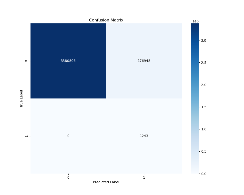
    # Create and plot confusion matrix
    plt.figure(figsize=(10, 8))
    cm = confusion_matrix(y_test, y_pred)
    sns.heatmap(cm, annot=True, fmt='d', cmap='Blues')
    plt.title('Confusion Matrix')
    plt.ylabel('True Label')
    plt.xlabel('Predicted Label')
    
    if fname:
        plt.savefig(f'results/confusion_matrix_{iteration}.png')
    else:
        plt.show()
    
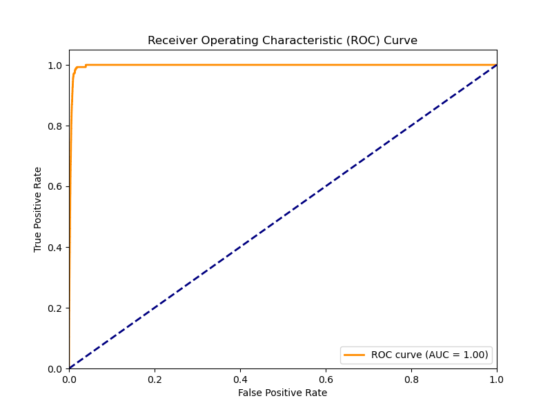
    # Plot ROC curve and calculate AUC
    plt.figure(figsize=(8, 6))
    fpr, tpr, _ = roc_curve(y_test, y_pred_proba)
    roc_auc = auc(fpr, tpr)
    
    plt.plot(fpr, tpr, color='darkorange', lw=2, 
             label=f'ROC curve (AUC = {roc_auc:.2f})')
    plt.plot([0, 1], [0, 1], color='navy', lw=2, linestyle='--')
    plt.xlim([0.0, 1.0])
    plt.ylim([0.0, 1.05])
    plt.xlabel('False Positive Rate')
    plt.ylabel('True Positive Rate')
    plt.title('Receiver Operating Characteristic (ROC) Curve')
    plt.legend(loc="lower right")
    
    if fname:
        plt.savefig(f'results/roc_curve_{iteration}.png')
    else:
        plt.show()
    
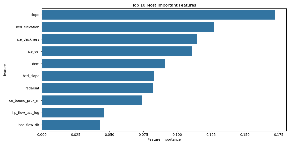
    # Create feature importance visualization
    if feature_names is not None:
        importance = pd.DataFrame({
            'feature': feature_names,
            'importance': clf.feature_importances_
        }).sort_values('importance', ascending=False)
        
        plt.figure(figsize=(12, 6))
        sns.barplot(data=importance.head(10), x='importance', y='feature')
        plt.title('Top 10 Most Important Features')
        plt.xlabel('Feature Importance')
        plt.tight_layout()
        
        if fname:
            plt.savefig(f'results/feature_importance_{iteration}.png')
        else:
            plt.show()
        
        return importance

def visualize_predictions_dual(results_gdf, min_probability=0.3, fname=False, iteration=None):
    """
    Create two-panel visualization comparing lake probabilities and prediction confidence
    
    Args:
        results_gdf: GeoDataFrame with prediction results
        min_probability: Minimum probability threshold for displaying predictions
    """
    # Create two-panel figure
    fig, (ax1, ax2) = plt.subplots(1, 2, figsize=(20, 8))
    
    # Filter to show only predictions above minimum probability threshold
    potential_lakes = results_gdf[results_gdf['lake_probability'] >= min_probability].copy()
    
    # Panel 1: Lake Probability
    # Plot low-probability points as background
    ax1.scatter(results_gdf[results_gdf['lake_probability'] < min_probability].geometry.x,
               results_gdf[results_gdf['lake_probability'] < min_probability].geometry.y,
               c='gray', alpha=0.1, s=1)
    
    # Plot predicted lakes colored by probability
    scatter1 = ax1.scatter(potential_lakes.geometry.x,
                          potential_lakes.geometry.y,
                          c=potential_lakes['lake_probability'],
                          cmap='viridis',
                          s=30,
                          alpha=0.7)
    
    # Highlight known lakes with red circles
    ax1.scatter(results_gdf[results_gdf['known_lake'] == 1].geometry.x,
                results_gdf[results_gdf['known_lake'] == 1].geometry.y,
                s=25, marker='o', label='Known lakes', alpha=0.3, facecolors='none', edgecolors='red')
    
    # Add colorbar and labels
    plt.colorbar(scatter1, ax=ax1, label='Lake Probability')
    ax1.set_title('Lake Probability Distribution')
    ax1.set_xlabel('X Coordinate (m)')
    ax1.set_ylabel('Y Coordinate (m)')
    ax1.legend()
    ax1.grid(True, alpha=0.3)
    
    # Panel 2: Prediction Confidence
    # Repeat similar plotting for confidence scores
    ax2.scatter(results_gdf[results_gdf['lake_probability'] < min_probability].geometry.x,
               results_gdf[results_gdf['lake_probability'] < min_probability].geometry.y,
               c='gray', alpha=0.1, s=1)
    
    scatter2 = ax2.scatter(potential_lakes.geometry.x,
                          potential_lakes.geometry.y,
                          c=potential_lakes['prediction_confidence'],
                          cmap='viridis',
                          s=30,
                          alpha=0.7)
    
    ax2.scatter(results_gdf[results_gdf['known_lake'] == 1].geometry.x,
                results_gdf[results_gdf['known_lake'] == 1].geometry.y,
                s=25, marker='o', label='Known lakes', alpha=0.3, facecolors='none', edgecolors='red')
    
    plt.colorbar(scatter2, ax=ax2, label='Prediction Confidence')
    ax2.set_title('Prediction Confidence Distribution')
    ax2.set_xlabel('X Coordinate (m)')
    ax2.set_ylabel('Y Coordinate (m)')
    ax2.legend()
    ax2.grid(True, alpha=0.3)
    
    plt.tight_layout()
    
    if fname:
        plt.savefig(f'results/spatial_predictions_{iteration}.png')
    else:
        plt.show()

Model Usage

for i in range(1): # iterative setup to test different parameters

    print(f'## Iteration {i} ##')

    print('## Creating Lake Prediction Model ##')
    clf, iso_forest, scaler, X_test, y_test = create_lake_prediction_model(df, features_to_exclude=['known_lake'], data_frac=0.1)
    print('## Model Created ##')

    print('## Predicting Potential Lakes ##')
    potential_lakes, probs, scores = predict_potential_lakes(df, clf, iso_forest, scaler, 
                                                            features_to_exclude=['known_lake'], similarity_threshold=0.3, anomaly_threshold=-0.4)
    
    print('## Analyzing Predictions ##')
    results = analyze_predictions(df, potential_lakes, probs, scores, iteration=i)

    # Evaluate model
    feature_names = df.drop(columns=['known_lake']).columns

    print('## Evaluating Model ##')
    importance_df = evaluate_model(clf, X_test, y_test, feature_names, fname=False, iteration=i)

    # Merge with geometry and create GeoDataFrame
    print('## Merging with Geometry ##')
    results = results.merge(merged['geometry'], left_index=True, right_index=True)
    results_gdf = gpd.GeoDataFrame(results, geometry='geometry')

    # visualize_predictions_dual(results_gdf, min_probability=0.3, fname=False, iteration=i)

results_known_lakes = results[results['known_lake'] == 1]
results_pred_lakes = results[results['potential_lake'] == 1]

fig, axes = plt.subplots(1, 3, figsize=(15, 5))
cols = ['lake_probability', 'terrain_uniqueness', 'prediction_confidence']
for i, col in enumerate(cols):
    ax = axes[i]
    
    # Calculate statistics
    stats_all = {
        'mean': results_gdf[col].mean(),
        'median': results_gdf[col].median(),
        'min': results_gdf[col].min(),
        'max': results_gdf[col].max()
    }
    
    stats_pred = {
        'mean': results_pred_lakes[col].mean(),
        'median': results_pred_lakes[col].median(),
        'min': results_pred_lakes[col].min(),
        'max': results_pred_lakes[col].max()
    }

    stats_known = {
        'mean': results_known_lakes[col].mean(),
        'median': results_known_lakes[col].median(),
        'min': results_known_lakes[col].min(),
        'max': results_known_lakes[col].max()
    }

    # Plot histograms
    ax.hist(results_gdf[col], bins=50, alpha=0.5, label='All', log=True, color='orange')
    ax.hist(results_pred_lakes[col], bins=50, alpha=0.5, label='Predicted Lakes', log=True, color='grey')
    ax.hist(results_known_lakes[col], bins=50, alpha=0.5, label='Known Lakes', log=True, color='blue')

    # Add title and legend
    ax.set_title(col)
    ax.legend(loc='upper right')
    
    # Create and add text blocks separately with different colors
    all_text = (
        f"All Data (orange):\n"
        f"  Mean: {stats_all['mean']:.2f}\n"
        f"  Median: {stats_all['median']:.2f}\n"
        f"  Range: [{stats_all['min']:.2f}, {stats_all['max']:.2f}]"
    )

    pred_text = (
        f"\n\nPredicted Lakes (grey):\n"
        f"  Mean: {stats_pred['mean']:.2f}\n"
        f"  Median: {stats_pred['median']:.2f}\n"
        f"  Range: [{stats_pred['min']:.2f}, {stats_pred['max']:.2f}]"
    )
    
    known_text = (
        f"\n\nKnown Lakes (blue):\n"
        f"  Mean: {stats_known['mean']:.2f}\n"
        f"  Median: {stats_known['median']:.2f}\n"
        f"  Range: [{stats_known['min']:.2f}, {stats_known['max']:.2f}]"
    )
    
    # Add text blocks with separate colors
    ax.text(0.05, 0.95, all_text,
            transform=ax.transAxes,
            verticalalignment='top',
            fontsize=8,
            family='monospace',
            color='orange',
            bbox=dict(facecolor='white', alpha=0.8))
            
    ax.text(0.05, 0.65, known_text,
            transform=ax.transAxes,
            verticalalignment='top',
            fontsize=8,
            family='monospace',
            color='blue',
            bbox=dict(facecolor='white', alpha=0.8))
 
plt.tight_layout()
plt.show()

To determine the binary classification of possible lake areas, I used a lake probability threshold of 0.4 and a terrain uniqueness threshold of -0.4.

These values were determined using trial and error as well as researched information on subglacial lakes.

My findings compared to those of Goeller S. et al. (2016) show that my model is more conservative in predicting subglacial lakes. This is likely due to the terrain uniqueness threshold I used.

My final prediction map.